I used to catalogue my holidays using Polarsteps. It's a great app for tracking your travels, sharing photos and keeping a journal as you go. But my organising tendencies cannot abide the minor but regular inaccuracies of the Polarsteps travel tracker.
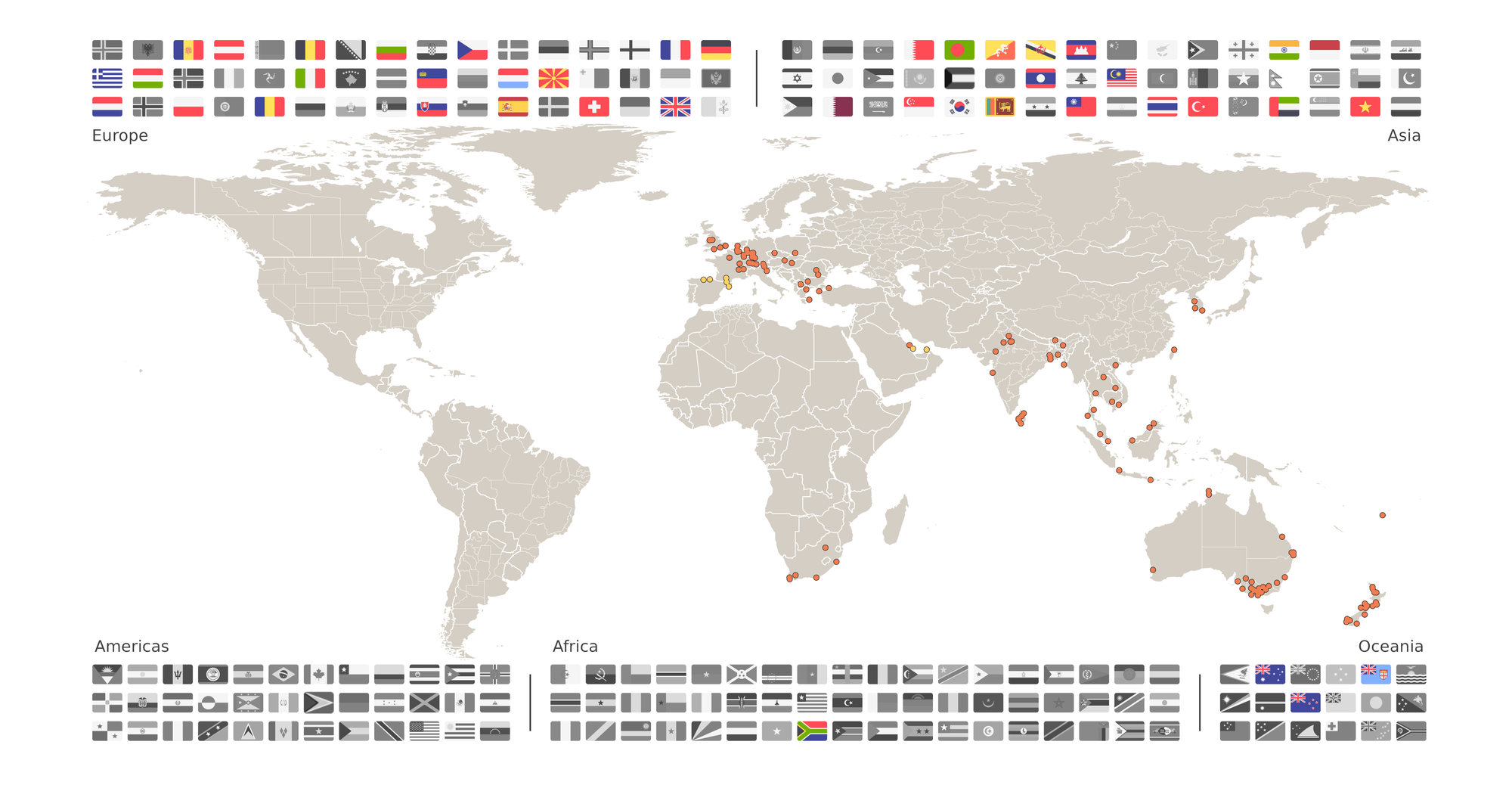
Instead, I built my own map in R that drops pins on the cities I've visited and colours in the flags of countries I've passed through. Here's the code I used to create this in R.
If you want to create something similar for yourself, read on.
Requisite files
You can update the destination list with your own travel destinations.
Setup
# Get github packages
devtools::install_github(
  repo = c(
    "ropensci/rnaturalearthhires",
    "ropensci/rnaturalearthdata"
  ),
  quiet = TRUE
)

# Load packages
pacman::p_load(
  char = c(
    "rnaturalearth",
    "countrycode",
    "tidyverse", # For everything
    "patchwork", # For better plot layout
    "here",
    "sf"
  )
)

# Pick the colours for the graph
graph_colours <- c(
  "Visited"        = "#F07C51",
  "Planned"        = "#FFCF66",
  "Travel_outline" = "#000000",
  "Country_fill"   = "#D4CEC4",
  "Border_line"    = "#FFFFFF"
)
Trips
Create trip data
df_locations <-
  googlesheets4::read_sheet(
    paste0(
      "https://docs.google.com/spreadsheets/",
      "d/1Ia0IhKe3eP0LEZnJn388VjA7dCtuVeC37WLFUPhhpLg/",
      "edit#gid=833795961"
    )
  ) %>%
  janitor::clean_names() %>%
  mutate(
    place_country = ifelse(
      is.na(place_country),
      paste(place, country, sep = ", "),
      place_country
    )
  )
Geocode trips
# Select any locations missing a lat or lon coordinate
df_geocodes <-
  df_locations %>%
  filter(is.na(lon) | is.na(lat)) %>%
  select(-starts_with(c("lat", "lon")))

# If there are any missing, then geocode them
if (nrow(df_geocodes) > 0) {
  df_geocodes <-
    df_geocodes %>%
    bind_cols(
      tmaptools::geocode_OSM(
        q = .$place_country,
        as.data.frame = T
      )[, c("lon", "lat")]
    )
}

# Join the two
df_locations <-
  df_locations %>%
  dplyr::rows_update(x = ., y = df_geocodes, by = "place_country") %>%
  arrange(status, continent, country)

# Clear the environment
rm(df_geocodes)
Save trip data
if (TRUE == FALSE) {
  write.csv(
    x = df_locations,
    file = paste0(here::here(), "/Output/Destinations.csv"),
    row.names = FALSE
  )
}
Flags
Read flags data
# Load dataframe I created earlier
df_flags <-
  read_csv(
    paste0(
      here::here(),
      "/Input/Flag Names.csv"
    )
  ) %>%
  janitor::remove_empty(
    which = c("rows", "cols"),
    quiet = TRUE
  )

# Remove countries, and put Serbia in alphabetical order
df_flags <-
  df_flags %>%
  filter(keep == TRUE) %>%
  select(-keep) %>%
  mutate(name = if_else(name == "Republic of Serbia", "Serbia", name))
Colour in visited flags
# Create columns
df_flags <-
  df_flags %>%
  mutate(
    visited = if_else(
      name %in% unlist(
        df_locations %>%
          filter(status %in% c("Visited", "Planned")) %>%
          select(country)
      ),
      TRUE,
      FALSE
    ),
    file_path = paste0(
      here::here(),
      "/Input/Flags/",
      if_else(visited == TRUE, "colour", "grey"), # Colour based on visited
      "/",
      file_name
    )
  )
Create grid references
# Create columns
df_flags <-
  df_flags %>%
  mutate(
    continent = if_else(
      str_detect(continent, "America"),
      "Americas",
      continent
    )
  ) %>%
  arrange(continent, name) %>%
  mutate(
    .by = continent,
    n_flags = n(),
    n_cols = n_flags / 3,
    x = rep(1:max(n_cols), 3),
    y = 3 - cumsum(n_cols == lag(x, default = 1)),
    y = if_else(continent %in% c("Europe", "Asia"), y + 22, y)
  ) %>%
  mutate(
    .by = y,
    row_fraction = 39 / (n() + n_distinct(continent) - 1),
    x = x * row_fraction - row_fraction,
    x = case_when(
      continent == "Asia" ~ x + row_fraction * 2 + 17.727273,
      continent == "Africa" ~ x + row_fraction * 2 + 11.289474,
      continent == "Oceania" ~ x + row_fraction * 4 + 11.289474 + 17.447368,
      TRUE ~ x
    )
  )

# Create df of continent names
df_names <-
  df_flags %>%
  summarise(
    .by = continent,
    x = if_else(
      continent %in% c("Asia", "Oceania"),
      max(x) + row_fraction / 2,
      min(x) - row_fraction / 2
    ),
    y = if_else(first(y) < 4, 4, 22),
    hjust = if_else(continent %in% c("Asia", "Oceania"), 1, 0)
  ) %>%
  ungroup() %>%
  filter(duplicated(.) == FALSE)

# Create a df of lines and text
df_lines <-
  df_flags %>%
  summarise(
    .by = continent,
    x = if_else(
      continent %in% c("Americas", "Africa", "Europe"),
      max(x) + row_fraction,
      NA
    ),
    xend = x,
    y = min(y),
    yend = y + 2
  ) %>%
  filter(duplicated(.) == FALSE)
Map
Download map data
# Download map data
df_world <-
  rnaturalearth::ne_countries(
    type = "countries",
    scale = "large",
    returnclass = "sf"
  ) %>%
  sf::st_make_valid()

# Remove Antarctica, Chile, Kazakhstan and small military bases
df_world <-
  df_world %>%
  filter(
    !name %in% c("Antarctica", "Chile", "Kazakhstan", "Baikonur"),
    !brk_a3 %in% c("B69", "CLP", "SGS", "HMD", "ATF", "SHN")
  )

# Restore removed map sections in the manner we need
df_world <-
  df_world %>%
  bind_rows(
    .,
    # Restore Chile with a lower resolution coastline
    rnaturalearth::ne_countries(
      type = "countries",
      country = "Chile",
      scale = "medium",
      returnclass = "sf"
    ) %>%
      sf::st_make_valid(),
    # Combine Baikonur with Kazakhstan
    rnaturalearth::ne_countries(
      type = "countries",
      geounit = c("Baykonur Cosmodrome", "Kazakhstan"),
      scale = "large",
      returnclass = "sf"
    ) %>%
      sf::st_make_valid() %>%
      mutate(geometry = sf::st_union(geometry)) %>%
      filter(name != "Baikonur")
  )
Download state borders
shapefile_dir <- here::here("Input", "States")

if (!dir.exists(shapefile_dir)) dir.create(shapefile_dir)

shapefile_dir_empty <- length(list.files(shapefile_dir)) == 0L

if (shapefile_dir_empty) {
  shapefile_zip <- here::here(
    shapefile_dir,
    "shapefile.zip"
  )

  download.file(
    paste0(
      "https://www.naturalearthdata.com/http//",
      "www.naturalearthdata.com/download/",
      "10m/",
      "cultural/",
      "ne_10m_admin_1_states_provinces_lines.zip"
    ),
    shapefile_zip
  )

  unzip(
    shapefile_zip,
    exdir = shapefile_dir
  )

  file.remove(shapefile_zip)
}

df_states <-
  sf::st_read(shapefile_dir) %>%
  janitor::clean_names() %>%
  filter( # Top 10 countries by area
    adm0_a3 %in% c(
      "CAN", "USA", "RUS", "KAZ", "CHN",
      "IND", "BRA", "AUS", "DZA", "ARG"
    )
  ) %>%
  select(name = adm0_name, geometry) %>%
  sf::st_make_valid()
Download great lakes
shapefile_dir <- here::here("Input", "Lakes")

if (!dir.exists(shapefile_dir)) dir.create(shapefile_dir)

shapefile_dir_empty <- length(list.files(shapefile_dir)) == 0L

if (shapefile_dir_empty) {
  shapefile_zip <- here::here(
    shapefile_dir,
    "shapefile.zip"
  )

  download.file(
    paste0(
      "https://www.naturalearthdata.com/http//",
      "www.naturalearthdata.com/download/",
      "10m/",
      "physical/",
      "ne_10m_lakes.zip"
    ),
    shapefile_zip
  )

  unzip(
    shapefile_zip,
    exdir = shapefile_dir
  )

  file.remove(shapefile_zip)
}

df_lakes <-
  sf::st_read(shapefile_dir) %>%
  filter(
    scalerank < 1 |
      name %in% c("Lake Chad", "Lago de Nicaragua", "Lake Onega")
  ) %>%
  select(-c(name_abb:name_zht)) %>%
  sf::st_make_valid()
Adjust projection
# Specify projection
target_crs <-
  sf::st_crs(
    paste0(
      "+proj=longlat ", # Projection
      "+lon_0=0 ",
      "+x_0=0 ",
      "+y_0=0 ",
      "+datum=WGS84 ",
      "+units=m ",
      "+pm=10 ", # Prime meridian
      "+no_defs"
    )
  )

# Specify 180 - the lon the map is centered on
offset <- 180 - 10 # lon 10

# Create thin polygon to cut the adjusted border
polygon <-
  sf::st_polygon(
    x = list(rbind(
      c(-0.0001 - offset,  90),
      c( 0.0000 - offset,  90),
      c( 0.0000 - offset, -90),
      c(-0.0001 - offset, -90),
      c(-0.0001 - offset,  90)
    ))
  ) %>%
  sf::st_sfc() %>%
  sf::st_set_crs(4326)

# Remove overlapping part of world and change projection
df_world <-
  df_world %>%
  sf::st_difference(polygon) %>%
  sf::st_transform(crs = target_crs)

df_states <-
  df_states %>%
  sf::st_difference(polygon) %>%
  sf::st_transform(crs = target_crs)

df_lakes <-
  df_lakes %>%
  sf::st_difference(polygon) %>%
  sf::st_transform(crs = target_crs)

# Clear environment
rm(polygon, target_crs, offset)
Graph
Create Travel Map
# Create map
graph_world <-
  ggplot() +
  ggplot2::geom_sf( # Countries
    data = df_world,
    fill = graph_colours["Country_fill"],
    colour = graph_colours["Border_line"],
    linewidth = 0.25
  ) +
  ggplot2::geom_sf( # State borders
    data = df_states,
    colour = graph_colours["Border_line"], # State border
    linewidth = 0.1
  ) +
  ggplot2::geom_sf( # Lakes
    data = df_lakes,
    fill = "#FFFFFF",
    colour = graph_colours["Border_line"],
    linewidth = 0.1
  )

# Add travel dots
graph_world <-
  graph_world +
  geom_point( # Back dots
    data = df_locations %>% filter(!status %in% c("Wish-list")),
    aes(x = lon, y = lat),
    colour = graph_colours["Travel_outline"],
    size = 1.25
  ) +
  geom_point( # Front dots
    data = df_locations %>% filter(!status %in% c("Wish-list")),
    aes(x = lon, y = lat, colour = status),
    size = 1
  ) +
  scale_color_manual(
    name = "",
    values = c(
      "Visited" = graph_colours[["Visited"]],
      "Planned" = graph_colours[["Planned"]]
    )
  )

# Crop the map
graph_world <-
  graph_world +
  ggplot2::coord_sf(
    expand = FALSE,
    default_crs = sf::st_crs(4326),
    xlim = c(-172, -169),
    ylim = c(90, -60)
  ) +
  theme(
    axis.text = element_blank(),
    axis.title = element_blank(),
    axis.ticks = element_blank(),
    panel.grid = element_blank(),
    panel.background = element_blank(),
    plot.background = element_blank(),
    legend.position = "none"
  )
Create Flag Backdrop
graph_flags <-
  ggplot() +
  nflplotR::geom_from_path(
    data = df_flags,
    aes(
      x = x,
      y = y,
      path = file_path
    ),
    height = 0.04
  ) +
  geom_segment(
    data = df_lines,
    aes(
      x = x,
      xend = xend,
      y = y,
      yend = yend
    ),
    colour = "grey25"
  ) +
  geom_label(
    data = df_names,
    aes(
      label = continent,
      x = x,
      y = y,
      hjust = hjust
    ),
    colour = "grey25",
    label.size = 0
  ) +
  theme(
    axis.text = element_blank(),
    axis.title = element_blank(),
    axis.ticks = element_blank(),
    panel.grid = element_blank(),
    panel.background = element_blank()
  )
Combine Graphs
graph_world_travel_flags <-
  graph_flags +
  patchwork::inset_element(
    p = graph_world,
    on_top = F,
    left = 0,
    right = 1,
    top = 0.9,
    bottom = 0.1
  )
Export
ggsave(
  plot = graph_world_travel_flags,
  path = paste0(here::here(), "/Output"),
  filename = "graph_travel_and_flags_A4.png",
  device = "png",
  dpi = 600,
  units = "cm",
  width = 36.6,
  height = 19.0
)