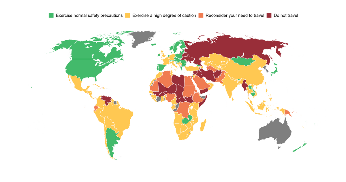
The Australian Government operates the site https://www.smartraveller.gov.au/ which advises Australians on whether and where to travel. Oftentimes the maps are down as the Government reconsiders its advice, but the overall travel advisory remains.
For those who want to create their own map, you can use the following code to web scrape the Smart Traveler website and plot the results in R.
Obviously this map isn't tailored to your needs and offers no guidance on travel within countries. Do your own research before traveling.
Setup
# Libraries
library(tidyverse)
library(rvest)
library(rnaturalearth)
library(tmaptools)
library(sf)

devtools::install_github(
  c("ropensci/rnaturalearthhires",
    "ropensci/rnaturalearthdata"))
Download data
# Web scrape Smartraveller.gov.au
df_smart_travel <-
  rvest::read_html("https://www.smartraveller.gov.au/destinations") %>%
  rvest::html_table() %>%
  as.data.frame()

# Fix formats
df_smart_travel <-
  df_smart_travel %>%
  janitor::clean_names() %>%
  rename(advice = overall_advice_level) %>%
  filter(advice != "") %>%
  mutate(
    updated = lubridate::parse_date_time(updated, "%d %b %Y"),
    advice = str_to_sentence(advice))

# Download map data
df_world <-
  rnaturalearth::ne_countries(
    type = "countries",
    scale = "large",
    returnclass = "sf") %>%
  sf::st_make_valid()

# Remove Antarctica, small overseas military islands and Chile
df_world <-
  df_world %>%
  filter(
    admin != "Antarctica",
    admin != "Chile", # Chile has complex island borders at high resolution
    !brk_a3 %in% c("B69", "CLP", "SGS", "HMD", "ATF", "SHN"))

# Add Chile back in lower at a resolution
df_world <-
  df_world %>%
  bind_rows(
    .,
    rnaturalearth::ne_countries(
      type = "countries",
      country = "Chile",
      scale = "medium",
      returnclass = "sf") %>%
      sf::st_make_valid()
  )

# Get great lakes
df_lakes <-
  rnaturalearth::ne_download(
    category = "physical",
    type = "lakes",
    scale = "large",
    returnclass = "sf") %>%
  filter(scalerank == 0) # Large lakes only
Clean data
# Keep only columns we need
df_world <-
  df_world %>%
  select(
    c(admin, geounit, name, name_long, formal_en, name_tr, adm0_a3), # Country names
    c(geometry) # Country shape
  )

# Add country travel advisory
df_all <-
  df_world %>%
  pivot_longer(
    cols = c(admin, geounit, name, name_long, formal_en, name_tr),
    values_to = "destination") %>%
  relocate("destination", everything()) %>%
  select(-name) %>%
  left_join(
    x = .,
    y = df_smart_travel,
    by = "destination") %>%
  filter(!is.na(geometry)) %>%
  distinct()

# Remove duplicates
df_all <-
  df_all %>%
  group_by(adm0_a3) %>%
  arrange(advice) %>%
  distinct(adm0_a3, .keep_all = T) %>%
  select(-adm0_a3)
Customise projection
# Specify projection
target_crs <-
  sf::st_crs(
    paste0(
      # Projection
      #"+proj=longlat ", #
      #"+proj=merc ", # Mercator, really messes up the antarctic
      "+proj=robin ", # Robinson
      "+lon_0=0 ",
      "+x_0=0 ",
      "+y_0=0 ",
      "+datum=WGS84 ",
      "+units=m ",
      "+pm=10 ", # Prime meridian
      "+no_defs"
    )
  )

# Specify 180 - the lon the map is centered on
offset <- 180 - 10 # lon 10

# Create thin polygon to cut the adjusted border
polygon <-
  sf::st_polygon(
    x = list(rbind(
      c(-0.0001 - offset,  90),
      c(0.00000 - offset,  90),
      c(0.00000 - offset, -90),
      c(-0.0001 - offset, -90),
      c(-0.0001 - offset,  90)))) %>%
  sf::st_sfc() %>%
  sf::st_set_crs(4326)


# Remove overlapping part of world
df_all <-
  df_all %>%
  sf::st_difference(polygon)

# Transform world projection
df_all <-
  df_all %>%
  sf::st_transform(crs = target_crs)

# Transform lake projection
df_lakes <-
  df_lakes %>%
  sf::st_transform(crs = target_crs)

# Clear environment
rm(polygon, target_crs, offset)
Create graph
# Graph the world
graph_world <-
  df_all %>%
  ggplot() +
  ggplot2::geom_sf(
    aes(fill = advice),
    colour = "#FFFFFF", # Country borders
    size = .2) +
  ggplot2::geom_sf(
    data = df_lakes,
    fill = "#FFFFFF",   # Lakes
    colour = "#FFFFFF", # Borders
    size = .2) +
  ggplot2::coord_sf(
    expand = TRUE,
    default_crs = sf::st_crs(4326)) +
  scale_fill_manual(
    values = c(
      "Exercise normal safety precautions" = "#43BA6B", # Green
      "Exercise a high degree of caution"  = "#FFC852",  # Yellow
      "Reconsider your need to travel" = "#F07C51", # Orange
      "Do not travel" = "#992E39")) + # Red
  theme(
    title = element_blank(),
    axis.ticks = element_blank(),
    axis.text.x = element_blank(),
    legend.justification = "centre",
    panel.grid.major = element_blank(),
    panel.background = element_rect(fill = "transparent"),
    plot.background  = element_rect(fill = "transparent", color = NA))
Print graph
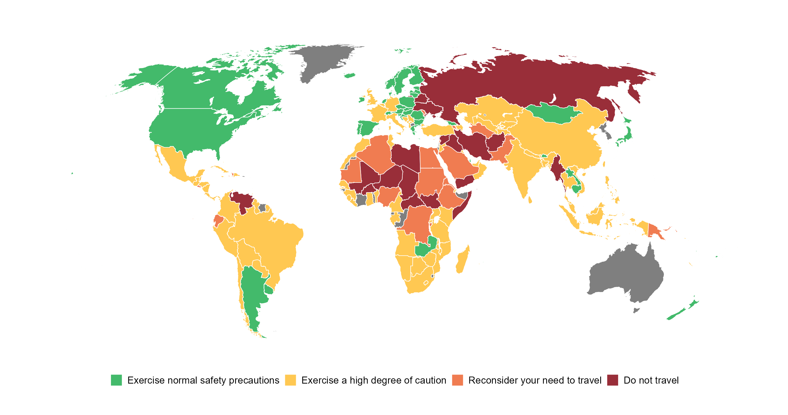
Future improvements
If you use this code, I suggest you try to apply the following improvements:
- Update the names of countries in
rnaturalearththat failed to match the Smart Traveler name: Suriname, South Korea, North Korea, Cote d'Ivoire, Togo, Congo, Somaliland, etc. - Update dependencies with higher-level advice, e.g. colour Greenland with the Denmark travel advisory, etc.
- If possible, colour in the Smart Traveler advice for regions within countries, not just the overall country advice.
- Increase the size of small island states, e.g. Cyprus, Micronesia, Fiji, etc.
- Apply a colour-blind friendly palette.